AIRS Frequency Calibration Notes
Tue, Nov 22, 20161 First Testing
1.1 Spectral Calibration Approach
The basic idea is to interpolate the observed spectra, say using the first-derivative of some fit to the BT spectrum, or
\begin{equation} BT = BT_o + \left(\frac{\partial BT}{\partial \nu}\right) \delta \nu \end{equation}where \(BT_o\) is the observed spectrum, \(BT\) is the spectrum on the desired fixed ν grid, and \(\delta \nu\) is the frequency offset of the observed data from the fixed grid.
Yibo generalized this equation by including two empirical parameters, \(a\) and \(b\)
\begin{equation} BT = BT_o + \left(a (\frac{\partial BT}{\partial \nu}) +b\right)\delta \nu. \end{equation}that are determined by least-squares fitting to simulated data. This is needed since it is difficult to derive a perfect expression for \((\partial BT/\partial \nu)\) from the data, especially since AIRS is not "Nyquist" sampled.
Yibo's approach for evaluating \((\partial BT/\partial \nu)\) is
\begin{equation} \frac{\partial BT}{\partial \nu} \equiv \frac{BT_o - BT_s}{\delta \nu} \end{equation}where \(BT_s\) is a spline fit to \(BT_o\) evaluated at the desired \(\nu\) grid. Plugging this into Eq. (2) gives you the existing JPL C-code algorithm,
\begin{equation} BT = (1-a) BT_o + a BT_s + b (\delta \nu) \end{equation}We have implemented a second approach, where we instead evaluate the derivative of the spline fit to the observed spectrum analytically, ie
\begin{equation} \left(\frac{\partial BT}{\partial \nu}\right) \equiv \left(\frac{\partial BT}{\partial \nu}\right)_{\text{Spline}} \end{equation}This approach might be less noise sensitive than Jibo's approach?
1.2 Approach
- Using Howard Motteler's algorithm for converting AIRS to CrIS ILS
- Deconvolve AIRS, reconvolve with shifted AIRS ILS functions (instead of CrIS ILS)
- Slightly better, especially in the longwave
- More computationally expensive?
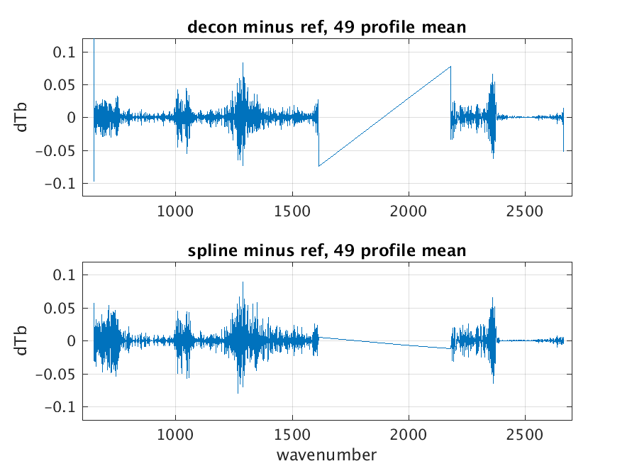
Figure 1: Calibration error using deconvolution/reconvolution vs spline interpolation. Data set is the RTA regression profiles.
1.3 Early Issue: Yibo's \(a,b\) are for 2378 Channel Set
Howard re-fit for \(a,b\) using 49 RTA regression profiles and tested against the same profiles (not independent) on L1c channel set.
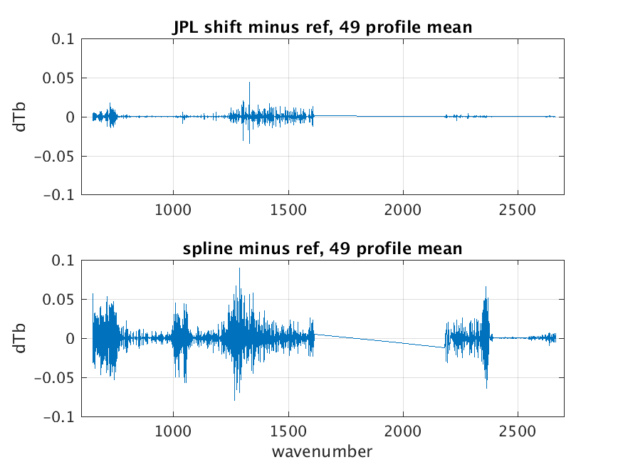
Figure 2: Calibration error for JPL a,b approach vs spline for 49 regression profiles.
1.4 New \(a,b\) Coefficients vs Old
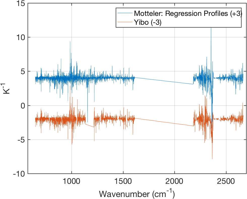
Figure 3: \(a\) Coefficients
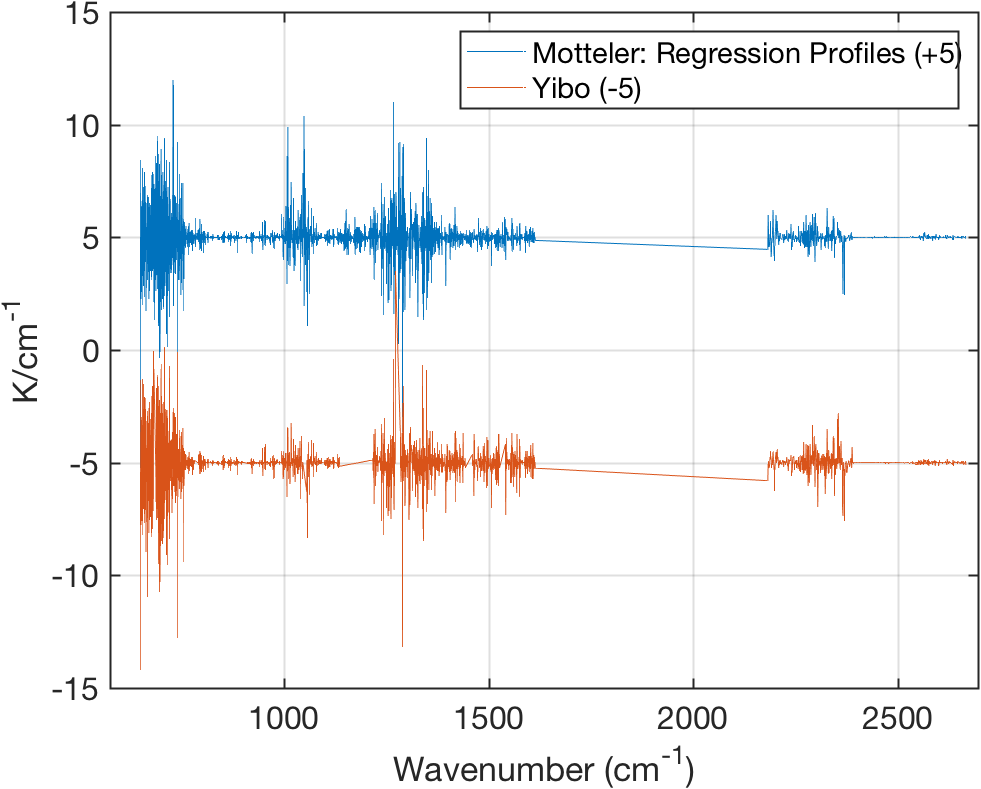
Figure 4: \(b\) Coefficients
Quite similar. Can be re-done using cloudy simulation data.
1.5 Single Spectrum Experiments: No Noise!
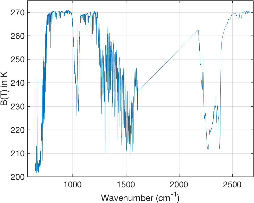
Figure 5: Sample simulated spectrum used for single scene testing.
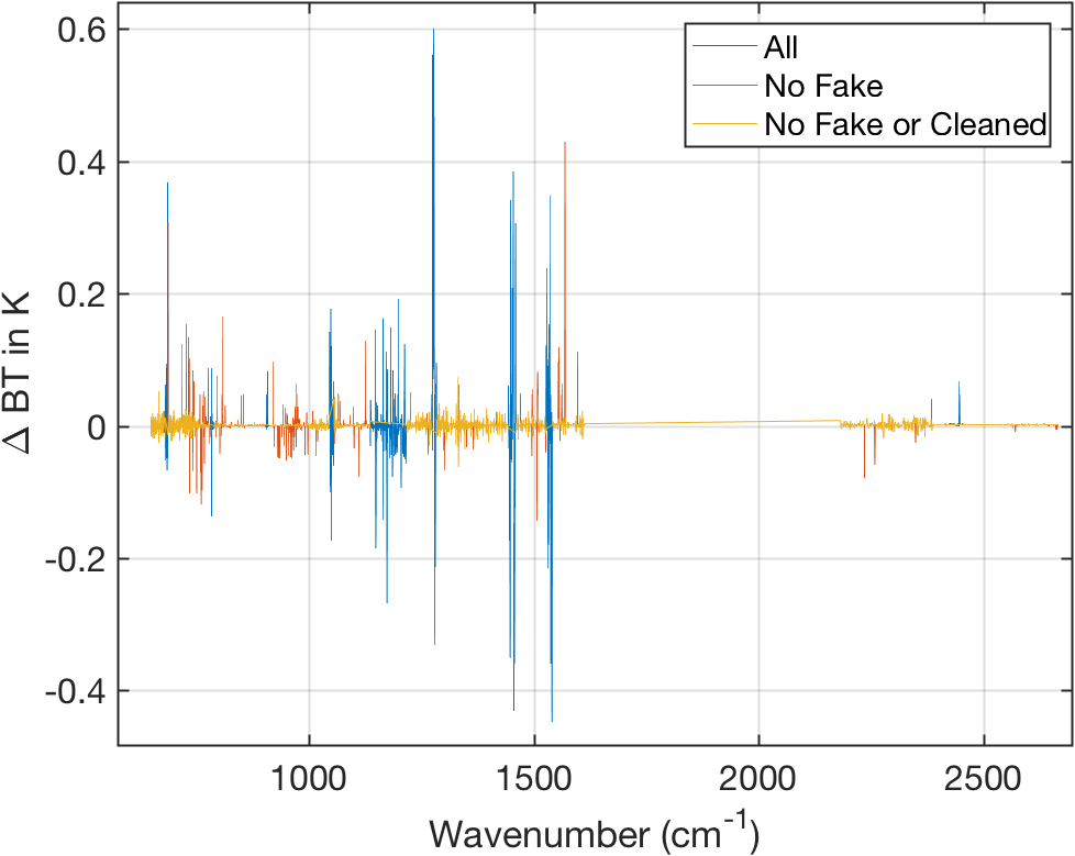
Figure 6: Calibration errors (JPL approach).
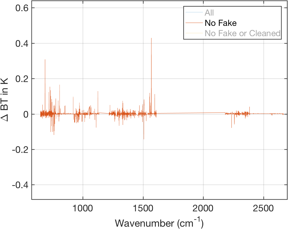
Figure 7: Same as above with fill channels removed.
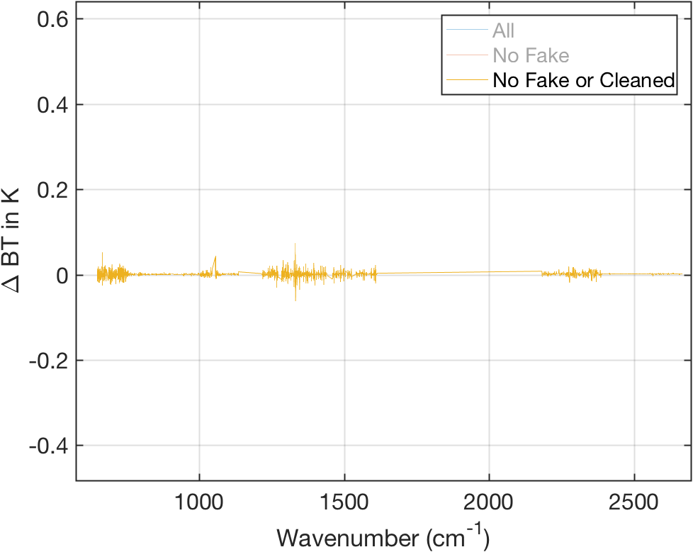
Figure 8: Same as above but also with cleaned channels removed.
1.6 Single Spectrum Experiments: With Noise
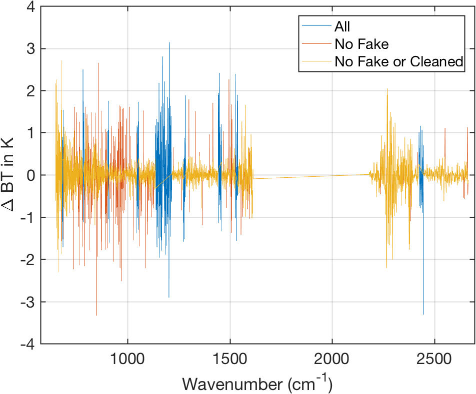
Figure 9: Single spectrum calibration errors (JPL approach) but with simulated noise.
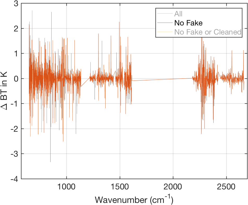
Figure 10: Same as above with fill channels removed.
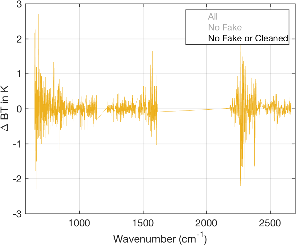
Figure 11: Same as above but also with cleaned channels removed.
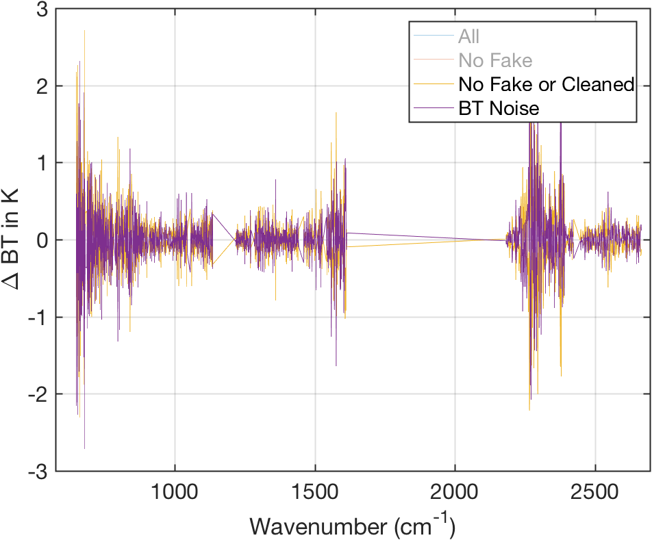
Figure 12: Comparison of (Obs-Cal BT) versus NeDT noise added to simulated spectrum.
1.7 Single Spectrum Experiments: \(\nu\) Calibration Noise
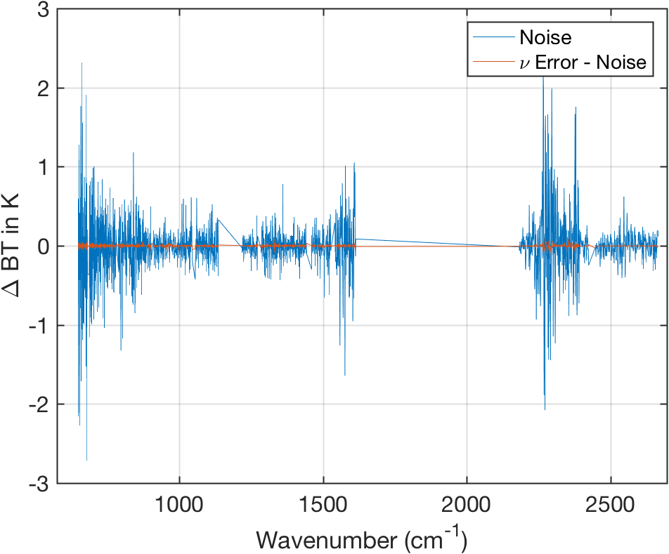
Figure 13: Comparison of scene noise to calibration error minus noise.
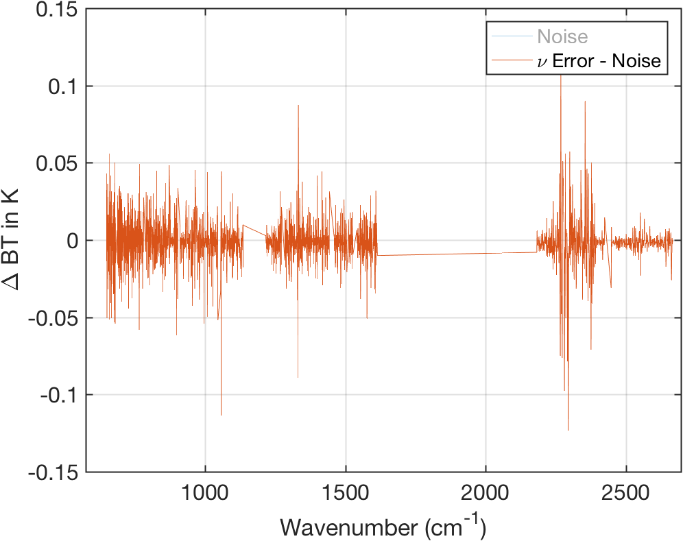
Figure 14: Same as above with scene noise removed.
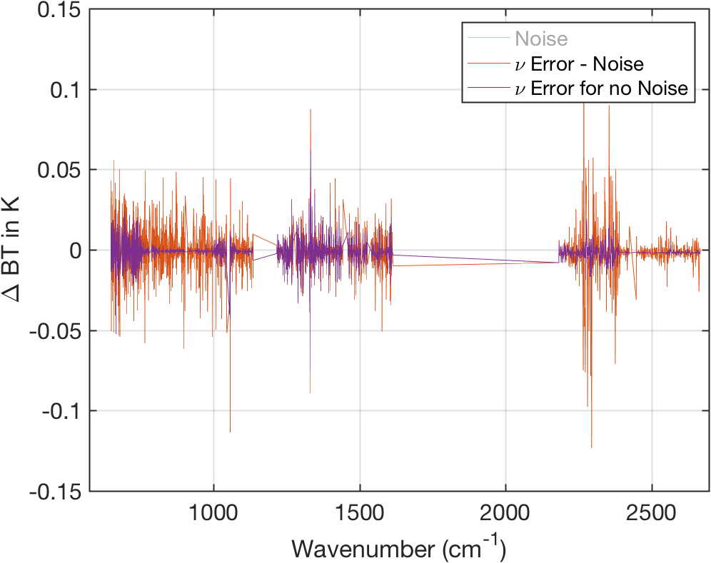
Figure 15: Calibration error (minus noise) compared to calibration error for case where no noise was added to the scene.
Appears that calibration is fairly insensitive to noise?
1.8 Comparison of Yibo vs Analytic Spline Derivative
- These results used a full granule
- Differences are smaller than absolute errors
- Statistical comparisons with truth too identical to call a winner
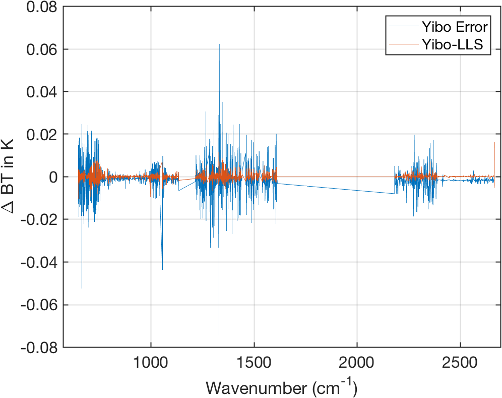
Figure 16: Yibo-Error is calibration error for granule average, using JPL calibration approach. Yibo-LLS is the difference between Yibo Error and calibration using spline analytic derivatives.
1.9 Results Using a Full Granule: Yibo approach
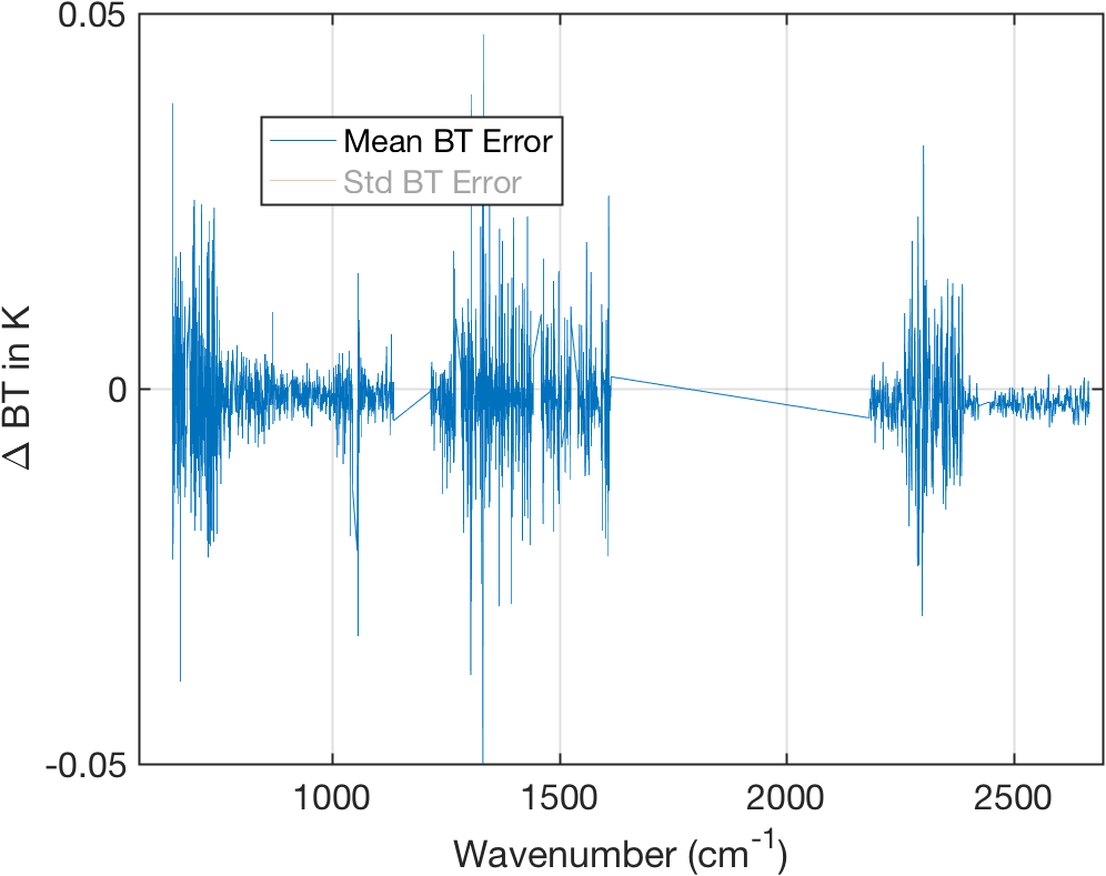
Figure 17: Full granule mean calibration errors (with noise) for JPL approach.
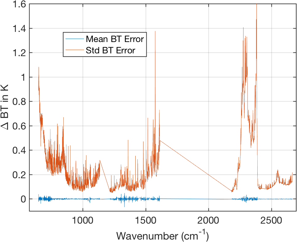
Figure 18: Same as above with standard deviation of calibration error.
Mean NedT - (Std Obs-Calc)
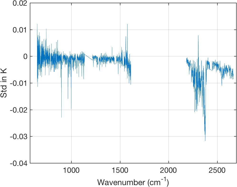
Figure 19: Mean NedT noise for graunle minu Std of (Obs - Calc) of calibration error.
- Calibration noise is detectable in the shortwave where curve goes below zero.
1.10 Conclusions
- Have derived \(a,b\) on L1c grid
- Yibo approach looks good, although fitting and testing with 1 micron only shifts.
- Probably re-fit \(a,b\) with simulated cloudy data and more shifts
- Analytic spline not worth the computation? (NOT CORRECT, always computed when fitting for splines.)
- Create a test day that cycles through full mission shifts, with Doppler?