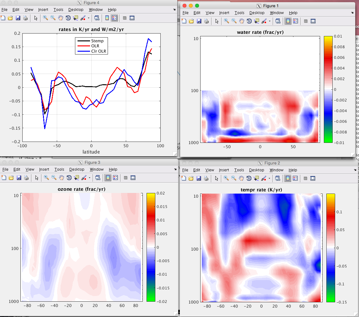
WV feedback from AIRS L3 data
Sun, Mar 13, 2016Location
** /home/sergio/MATLABCODE/ROSES_2013_GRANT/BT1231_pdfs_from_AIRSL3/read_in_airsL3.m **
13 year rates 2002/09-2015/08

The clear sky RTA is
$r(\nu) = \epsilon(\nu) r_{S}(\nu) exp(-k_{total}) + \sum B(T(i)) (1-exp(-k_{i})) \tau(i+1 \rightarrow N)$
for a window channel with minimal WV absorption, this can be approximated as
$r(\nu) = \epsilon(\nu) r_S(\nu) exp(-k_{total}) + B(A) (1-exp(-k_{total})) $
where $A$ is the effective atmospheric temperature and $k_{total}$ is the effective WV optical depth. So we have a suface emission that depends on surface temperature and total optical depth, and an atmospheric term which depends on the same total optical depth and an effective atmospheric temperature
What we have from AIRS L3 or ERA/ECM are estimates of the T(i),WV(i) and stemp. So what we can do is run SARTA CLEAR for the 1231 cm-1 channel in two modes
- with all the profile info, including surface temp
- turning off stemp
When I run sarta with and without stemp, I get the full $r(\nu)$
plus the $r_{atm}(\nu)$ assuming emissivity is 1 then subtracting
the two gives me $r_{S} \times e^{-k_{total}}$
Since$r_{S}$ is from the known surface temp, I effectively have the $k_{total}$
Going back to the second equation, I can now find $B(A)$ and hence the effective atmospheric temperature $A$.
I have gridded the AIRS L3 products into 36 latitude bins, (12 months x 13 years) of data and looked at all the tropical data, run through SARTA in the two modes described above. This gives me a handle on the surface temperature and on the “effective optical depth”.
I then looked at 2002/09 to 2004/08 and 2013/09 to 2015/08 data, and plotted 2d histograms as a function of surface temperature. In addition I plotted the means of the pdfs, and I see what I think is the Clausius-Clapeyron equation, plus an increase in optical depth of the water between the two times, as a function of surface temperature

Solid curves are the means of the 2d histograms, while the colorbar denotes how the 2d histograms have changed between 2002/2004 to 2013/2015
The left plot shows how for a given surface temperature the column water has increased between 2002/2004 to 2013/2015, while the right hand plot shows how the effective air temperature has also slightly gone up.
(Looking at the tropical AIRS L3 WV column amount between 2002-2015, that has definitely increased.)

Same plot as above, but now I have put in effective WV OD derived as discussed above. Sure looks exponential as stemp increases! Note the ODs are very reasonable, when compared to kCARTA ODs for a tropical profile.
Quick and dirty tropical linear stemp and col water rates are 0.003991 K/yr and 0.065645 mmW/yr
Maybe the conclusion is that the effective tropical atmospheric temperatures have gone up, so amount of tropical water vapor has gone up? Latter is consistent with WV L3 rates plot at top of page, former is a little stretch of the imagination.
PDFs
Doing pdfs of BT1231 calcs (or obs), Stemp and BT_Airs on the same temperature grid are quite easy. Making a pdf of the derived optical depth is also easy, but need to try to put it in a temperature context. So here is what I tried.
we have multiple ODs and stemps, as well as BT1231 calcs. Bin the ODs into M bins, and the stemps into N bins. Then looping over $(k)$ bins and $(stemp)$ bins, I can find the <BT1231> calc that corresponds to a $(k,stemp)$ pair, which allows me to build a matrix $C$ of size $N \times M$. This means
$pdf(k,dstemp) = C \times pdf(k,dk) $
where the optical depth $pdf(k,dk)$ in original $k$ space of size $M \times 1$ is transformed into a histogram $pdf(k,dstemp)$ in temperature space of size $N \times 1$ via the $N \times M$ matrix $C$.
So then I just computed the pdfs for the first two years vs the last two years. Plot below shows the pdfs for BTcalc (red), surface temp (black), retrieved air temperature (blue) and finally in green is the retrieved optical depth (in BT space). The lfeft plot are the pdfs (solid = 2002, dashed = 2014) while the right plots are the changes in pdfs.
Looks like a positive change in stemp (black curve) correlates decently well
with a positive change in OD (green curve), and vice versa

Below is the same set of plots, but for the Ch 1285
